The formula is the easy part. Two teams can report different cover for the same style on the same day and both be arithmetically correct, because cover depends on a choice nobody writes down: which weeks of sales go into the average. This article fixes the definition, shows what the choice does to the number, and gives the DAX that puts it in a Power BI model.
What Weeks of Cover Measures in Retail
Weeks of cover answers one question: how long will the stock last. It is also called weeks of supply, and in most retail teams the two terms are interchangeable.
What makes it useful is that it is stated in time, not in units or money. Four thousand units of stock means nothing without a sales rate behind it. Ten weeks of cover in week 12 of a twelve-week season means the range will not clear, and everyone in the trading meeting understands it in the same second.
Cover is a forward-looking read on stock built out of backward-looking data. That is exactly where it goes wrong.
The Weeks of Cover Formula and a Worked Example
Two decisions sit inside that line. The first is which stock: closing stock for the week being reported, or opening stock for the week ahead. Closing stock is the normal choice for a trading report, because that is what you have when the meeting starts. Planning guidance from Toolio writes the formula with beginning-of-period inventory, which is the same number shifted by one week. What matters is that one definition is used everywhere. The second decision is which weeks of sales, and it is the subject of the next two sections.
A worked example. One style, 1,200 units received, twelve weeks on sale. The figures are illustrative, chosen to show a normal decay curve.
| Week | Units sold | Closing stock |
|---|---|---|
| Week 1 | 180 | 1,020 |
| Week 2 | 150 | 870 |
| Week 3 | 120 | 750 |
| Week 4 | 95 | 655 |
| Week 5 | 80 | 575 |
| Week 6 | 70 | 505 |
| Week 7 | 55 | 450 |
| Week 8 | 45 | 405 |
| Week 9 | 40 | 365 |
| Week 10 | 30 | 335 |
| Week 11 | 25 | 310 |
| Week 12 | 20 | 290 |
In week 12 the style has 290 units left. Over the last four weeks it sold 115 units, 28.75 a week, so cover is 10.1 weeks. Over the whole season it sold 910 units, 75.8 a week, so cover is 3.8 weeks. Same stock, same week, same formula, and the answer differs by a factor of 2.6.
Choosing the Rate of Sale Window for Weeks of Cover
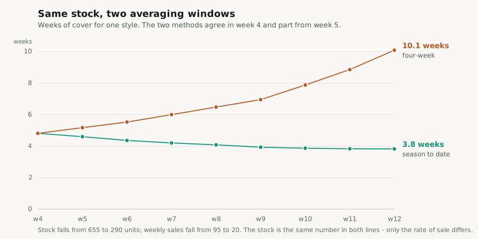
The two lines start on the same number in week 4 and never meet again. The reason is in the sales curve, not in the stock: demand decays, and a long window keeps feeding the average with the high early weeks.
That gives a rule worth remembering in both directions. On a declining curve, a long window hides overstock: season-to-date cover says 3.8 weeks, which reads as comfortable, while the style is actually selling 20 units a week and will not clear. On a rising curve, the same arithmetic in reverse hides a stockout, because the average lags the acceleration, cover looks longer than it is, and nobody raises the replenishment.
In a weekly trading report, a four-week rate of sale is the sane default. It is short enough to follow the trend and long enough to survive one odd week of weather or a promotion; Toolio's worked examples use four-week and eight-week trailing averages for the same reason. Season-to-date has one good use: judging how a whole range performed after it has finished.
Whichever window you pick, put it in the column header. Cover (4wk) is a measure. Cover is an argument waiting to happen.
Why Out-of-Stock Weeks Must Leave the Rate of Sale
A week in which a size ran out on Tuesday is not a week of demand. Leave it in the average and the rate of sale drops, cover rises, and the report recommends holding stock of something that was selling faster than you think.
The fix is to average over in-stock weeks only. Toolio puts the size of the error at roughly 30% or more of demand understated when zero-inventory weeks are included. Treat that as an order of magnitude rather than a constant, because it depends entirely on how often you break.
This is the correction most home-built cover reports are missing, and it is why the measure below counts its weeks instead of dividing by a fixed four.
A Weeks of Cover DAX Measure for Power BI
Three measures. The model is a star schema: a Date table, a Sales fact at day or week grain, and a Stock snapshot with one row per product, location and date.
Closing stock is semi-additive, which means it does not sum over time. Stock adds up across stores and styles, but across weeks you want the last value, not the total. The measure below takes the last date that actually has a snapshot, so it survives a model where stock is loaded weekly rather than daily. It follows the first-and-last-date-with-data pattern published by DAX Patterns; ALLEXCEPT is what makes every row of the matrix and the total agree on one date instead of each finding its own.
Closing Stock Units =
VAR MaxStockDate =
    CALCULATE (
        MAX ( Stock[Date] ),
        ALLEXCEPT ( Stock, 'Date' )
    )
VAR Result =
    CALCULATE (
        SUM ( Stock[Units] ),
        'Date'[Date] = MaxStockDate
    )
RETURN
ResultThe rate of sale builds the window with DATESINPERIOD, turns it into a list of weeks with VALUES, and drops the weeks that closed with no stock. Dividing by COUNTROWS of what survives is what keeps a broken week from diluting the average.
Rate of Sale 4W =
VAR WeeksBack = 4
VAR LastDay = MAX ( 'Date'[Date] )
VAR Window =
    DATESINPERIOD ( 'Date'[Date], LastDay, - WeeksBack * 7, DAY )
VAR WeeksInWindow =
    CALCULATETABLE ( VALUES ( 'Date'[Week Key] ), Window )
VAR InStockWeeks =
    FILTER ( WeeksInWindow, [Closing Stock Units] > 0 )
VAR UnitsSold =
    CALCULATE ( [Sales Units], InStockWeeks )
RETURN
DIVIDE ( UnitsSold, COUNTROWS ( InStockWeeks ) )Cover itself is then one line.
Weeks of Cover 4W =
DIVIDE ( [Closing Stock Units], [Rate of Sale 4W] )
Use DIVIDE rather than the division operator. When the rate of sale is zero, because the style sold nothing in the window, DIVIDE returns blank, and blank is the honest answer: stock that is not selling has no finite cover. Microsoft's guidance is to prefer DIVIDE for exactly this case and to leave the blank alone instead of passing a third argument that turns it into a zero. A zero would sort next to the fastest sellers in the range and get read as no stock problem.
One display decision belongs in the report rather than the model. Cover of 180 weeks and cover of 900 weeks carry the same message, so cap the visual at a number the business recognises and keep the blank visible as its own state.
Weeks of Cover (capped) =
VAR Cover = [Weeks of Cover 4W]
RETURN
IF ( ISBLANK ( Cover ), BLANK (), MIN ( Cover, 52 ) )How Weeks of Cover Converts to Stock Turn
Cover and stock turn are the same fact in two units. Four turns a year is thirteen weeks of average cover; thirteen weeks of average cover is four turns. This is worth knowing because the two numbers are usually owned by different people: the finance review talks in turns, the Monday trading meeting talks in weeks, and the conversion stops the two from drifting into separate versions of the truth.
The identity holds on averages across a year. Do not apply it to a single week of a seasonal range.
Forward Weeks of Cover for Seasonal Ranges
Backward-looking cover breaks on anything with a season, because the next four weeks will not look like the last four. For a coat in week 40, history understates what is coming; for the same coat in week 2, history overstates it badly.
In DAX this is the same measure with the forecast table in place of the sales fact. The decision is organisational rather than technical: forward cover is only worth building if a weekly forecast exists and somebody owns it. A forward cover driven by a forecast nobody maintains is worse than a trailing average, because it carries the same authority with none of the evidence.
Weeks of Cover Targets by Category
There is no universal target. Cover is right when it matches lead time, season length and how much risk the business will carry, and all three are yours rather than the industry's.
Two anchors help. The first is arithmetic: a minimum cover below the replenishment lead time guarantees a stockout, so the floor is lead time plus a buffer, which Toolio's planning guidance puts at about 25% — an eight-week lead time gives a ten-week minimum. The second is the turn benchmark converted with 52 ÷ turns.
| Category | Annual turns | Implied weeks of cover |
|---|---|---|
| Footwear | 3–5× | 10–17 |
| Apparel and fashion | 3–4× | 13–17 |
| Sporting goods | 3–4× | 13–17 |
| Home and furniture | 2–3× | 17–26 |
| Luxury and jewellery | 1–2× | 26–52 |
Read these as the shape of the distribution, not as a target to hit. They are one vendor's published figures, they cover whole categories rather than your channel mix, and an own-brand retailer with an eighteen-week critical path has a different floor from a wholesaler buying in season.
Five Mistakes That Make Weeks of Cover Wrong
- Summing stock over weeks. Without a semi-additive measure, a quarter column adds thirteen weekly snapshots together and reports cover of several years.
- Leaving out-of-stock weeks in the rate of sale. Demand is understated, cover is overstated, and the replenishment goes to the wrong styles.
- Mixing the windows. A four-week cover on one page and a season-to-date cover on another, both labelled cover, produce two true numbers and one argument.
- Turning the blank into a zero. Non-sellers then sort with the best performers and disappear from the markdown list.
- Averaging cover across styles. The average of a cover column is not the cover of the range: divide total stock by the total rate of sale instead, which is what these measures already do at every level.